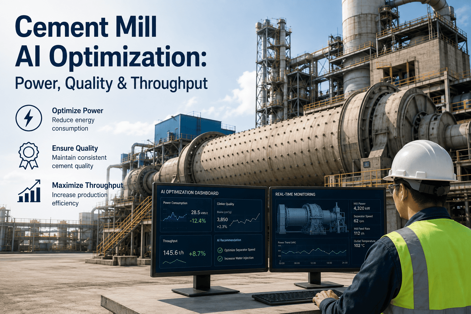
Cement Mill AI Optimization: Power, Quality & Throughput

A cement mill has three masters and they do not agree. Push throughput and specific power climbs. Chase the lowest kWh per tonne and Blaine drifts wide. Tighten quality and operators grind a safety margin above specification that quietly burns energy on every tonne shipped. Human operators resolve this conflict the only way they can — conservatively, on setpoints established at commissioning and adjusted by feel against a laboratory result that is already an hour old. AI optimization resolves it differently: by predicting where all three objectives land before the setpoint moves, and holding the balance every thirty seconds instead of every shift. See how this runs on a live grinding circuit with the iFactory deployment team.

The Three-Way Conflict At The Heart Of Every Grinding Circuit

Cement grinding is the single most energy-intensive operation in the production chain, consuming between 60 and 70 percent of a plant's total electrical demand — and only 1 to 5 percent of that energy performs actual particle size reduction. The rest becomes heat, noise and vibration. That is thermodynamics, not a design defect. What is a defect is how much of the remaining controllable margin gets given away because the control strategy can only chase one objective at a time.

Every setpoint move a mill operator makes trades one objective against another. Raise feed rate and throughput rises while residence time falls, so fineness drops and the separator has to work harder. Raise separator speed to recover fineness and recirculating load climbs, mill power rises, and the throughput gain evaporates. Grind finer than the specification requires and quality risk disappears — along with a meaningful slice of margin, because energy consumption rises exponentially with fineness rather than linearly. Grinding to 4,000 cm²/g consumes roughly 30 percent more energy than 3,200 cm²/g, and most plants routinely over-grind by 200 to 400 cm²/g purely as a safety buffer.

The Information Gap Operators Are Asked To Work Inside

Ask a control room operator why the mill is running two hundred points above target Blaine and the honest answer is simple: they cannot see fineness. Traditional Blaine testing requires hourly laboratory sampling, and during that hour the mill produces hundreds of tonnes on judgement alone. Clinker hardness shifts, gypsum moisture changes, ambient humidity moves, and the product drifts out of specification before the lab result arrives to confirm it. By the time the number lands, the material it describes is already in the silo.

This is why conservative operation is rational behaviour rather than poor practice. If you cannot measure the thing you are controlling until an hour after you controlled it, the only safe strategy is to over-shoot the target. The cost of that safety is not visible on any single shift report — it is spread thinly across every tonne, which is exactly why it survives audit after audit.

What The Optimiser Is Actually Moving

Multi-objective control does not mean the AI takes over the mill. It means a defined set of continuous variables is solved together against a weighted objective function, rather than adjusted one at a time by whoever is on shift. The variables below are the standard control surface for a cement finish grinding circuit. The bars indicate how strongly each one typically drives the optimisation outcome — research applying SHAP analysis to industrial vertical roller mill data confirmed that working pressure and input gas flow carry the highest importance for output temperature and motor power respectively, while for ball mills feed rate control combined with media grading consistently produces the largest measurable gains.

How The Closed Loop Actually Works

The architecture is less exotic than the term AI suggests. Plant data flows in from the existing DCS, PLC and SCADA layer. Predictive models estimate the variables nobody can measure in real time. An optimiser solves the weighted objective across all controllable variables at once. Recommended setpoints go back — either to the operator as an advisory, or directly to the control system as a write, depending on the mode the plant has authorised.

The critical property of this loop is that it closes. A recommendation engine that produces a report nobody acts on changes nothing, which is why the gap between advisory and autonomous operation is so consequential — McKinsey research documented up to 10 percent throughput and efficiency improvement in autonomous AI mode compared with advisory-only deployment. Most plants begin in advisory mode to build operator trust, then move loop by loop to closed-loop control once the recommendations have been observed to be sound.

Soft Sensors: Measuring What Cannot Be Measured

A soft sensor is a model that infers a variable you cannot instrument directly from variables you can. In cement grinding, they are the piece that makes real-time optimisation possible at all, because the two numbers that matter most — fineness and strength — arrive from a laboratory hours or days after the material was made. AI models map the relationship between mill operating parameters such as power draw, elevator current, separator speed, load signals and vibration against historical laboratory results, and after training on one to three years of plant data these virtual sensors predict fineness every few seconds with correlation above 0.95.

The effect on quality control is direct. When fineness becomes visible continuously rather than hourly, the safety margin can be reduced without increasing risk, and reported outcomes include Blaine standard deviation dropping by up to 60 percent under AI control. Tighter variance is what allows the target to move down toward specification minimum, and that move is where the energy saving is actually realised.

What This Looks Like In The Control Room

Operators do not interact with an optimiser through a model. They interact through plain language, and the most common question during the first weeks of deployment is not what to do but why.

That exchange is the whole product in miniature. The AI explains its reasoning in process terms, quantifies the trade-off before the change is made, respects the constraint the operator sets, and defines its own revert condition. Explainability is not a compliance feature here — it is the mechanism by which a control room decides to trust closed-loop operation.

What Ships, And What We Do On Site

The most common objection to mill AI is not technical scepticism — it is the assumption that adopting it means a multi-year IT project, a server room build, a data engineering hire and a rip-and-replace of the control system. None of that is the case. The platform is delivered as a turnkey bundle: hardware and software together, pre-configured before it leaves us, and integrated with the DCS, PLC and SCADA you already run.

Live In 6 To 12 Weeks: The Three-Phase Roadmap

Deployment is sequenced so the plant sees value before it grants control. Nothing is written to the DCS until the models have been observed predicting correctly against your own laboratory results, on your own clinker, for weeks.

Where The Numbers Land

The returns from mill AI are not speculative, but they are specific to the circuit. A mill already running close to its optimum has less to recover than one operating on commissioning setpoints and a wide quality buffer, which is why every serious deployment starts with a measured baseline rather than a promised percentage.

What The AI Does Not Touch

Trust in a control room is built on limits, not on capability claims. A plant needs to know precisely where the boundary sits before it authorises anything to write to a live circuit, so the boundary is defined in the deployment scope rather than discovered later.

Frequently Asked Questions