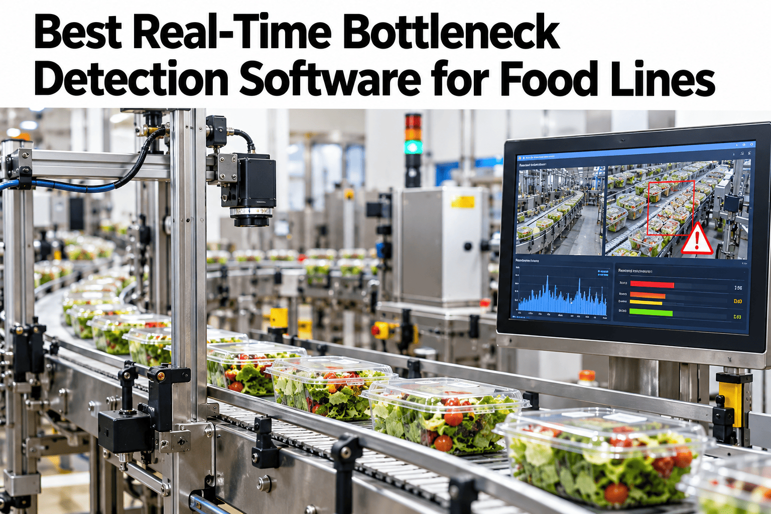
The constraint on a food production line is almost never fixed in one place. A filler that limits throughput on the morning shift running a thin sauce can become irrelevant by afternoon once the line switches to a thicker product and the capper becomes the real limiter instead. A static capacity study, run once and filed away, captures exactly one version of a line that keeps changing shift to shift and SKU to SKU, which is why it stops being useful almost as soon as it is finished. Plants that want to see where their actual constraint sits right now, not where it sat during last quarter's study, can watch a live constraint reading on their own line.
Your Bottleneck Moves. Your Capacity Study Doesn't.
iFactory AI reads accumulation, starvation and blocking live, so food plants see which station is the real constraint right now, not which one was the constraint during last quarter's study.
Why a One-Time Capacity Study Expires Fast
Ask a plant engineer which station is the bottleneck and they will usually give a confident answer, often based on the study that originally commissioned the line or justified the last capital project. That answer was likely accurate at the time, but lines rarely stay static. New SKUs get added, crews rotate, and small mechanical adjustments accumulate over months, each one nudging a station's effective speed slightly without anyone running a fresh study to confirm the constraint has not moved.
A traditional capacity study captures a snapshot: this line, this product, this shift, this day. The moment any of those variables changes, a different SKU, a different crew, a different ambient temperature affecting viscosity, the snapshot stops reflecting reality. Most plants keep acting on a study that was accurate the day it was run and has been drifting out of date ever since.
Reading Accumulation, Starvation and Blocking
The constraint on a line always leaves a visible signature in the stations around it, even when nobody has formally measured it. Product piles up just before the slow station and runs thin just after it. Learning to read those signatures live is what replaces a static study with a continuously accurate picture.
Find Your Real Constraint, Not Last Quarter's
Book a 30-minute session and see iFactory AI read accumulation, starvation and blocking on your own line in real time.
Why the Constraint Moves Between Shifts
A line running the same product can still show a different constraint from shift to shift, usually because the crew's pace and experience level affects how close each station runs to its theoretical capacity. A less experienced crew on a station that normally has slack can turn that station into the real constraint for the duration of their shift, even though the equipment itself has not changed at all.
| Shift | Constraint Station | Likely Driver |
|---|---|---|
| First shift | Capper | Experienced crew runs filler near rated speed, exposing capper as the ceiling |
| Second shift | Filler | Newer crew runs filler conservatively, masking the capper's true limit |
| Third shift | Labeler | Reduced staffing slows label roll changes, shifting the constraint downstream |
What Gets Missed When Nobody Is Watching Between Stations
Most plant floor attention naturally focuses on the stations themselves, since that is where the equipment and the operators are. The space between stations, the buffer or accumulation zone, tends to get far less attention, even though it is exactly where the constraint signal first appears. A supervisor walking the floor will notice a stopped machine immediately but may not register that product has been slowly piling up in a buffer for the last twenty minutes.
That blind spot is precisely why constraint identification benefits from continuous automated reading rather than relying on floor observation alone. The signal exists well before a human would typically notice it, simply because nobody is specifically watching the space between stations as their primary job.
Why the Constraint Moves Between SKUs
Product mix affects the constraint just as much as crew does, sometimes more. A thin, free-flowing product moves through a filler quickly but can overwhelm a labeler sized for a different bottle shape. A thick product does the opposite, slowing the filler while leaving plenty of slack downstream.
Viscosity
Thicker products slow fill rate, often shifting the constraint upstream toward the filler.
Bottle or Container Geometry
An unusual shape can slow a labeler or cartoner that handles standard formats quickly.
Fill Volume
Larger fill volumes extend cycle time at the filler proportionally more than at downstream stations.
Cap or Closure Type
A more complex closure can turn the capper into the constraint for specific SKUs only.
A Composite Day: The Constraint in Motion
The scenario below reflects an illustrative day on a beverage line, tracking where accumulation signals pointed to the real constraint across three different production runs.
Why Theory of Constraints Still Applies, With a Live Twist
The underlying logic of Theory of Constraints, that a system's output is governed by its single weakest link and improving anything else does not raise total throughput, has not changed. What has changed is the ability to identify that weakest link continuously instead of through a periodic study, which means the classic advice to "find the constraint, exploit it, then elevate it" can now be applied against a target that is actually current.
Exploiting a constraint identified three months ago, when the real constraint has since moved, wastes the exploitation step entirely. Live detection keeps the classic method pointed at the station that actually matters today.
Building the Case Across Engineering and Production
A real-time bottleneck detection program touches how engineering prioritizes capital projects and how production schedules its improvement focus differently, and each group tends to ask a different question before trusting a live constraint reading over a static study.
Where iFactory AI Fits
Reading accumulation, starvation and blocking continuously, across every station, shift and SKU, requires sensor data and flow analysis running live rather than a periodic manual study. iFactory AI reads those signals in real time and surfaces the current constraint automatically, so the answer to "where's our bottleneck" stays accurate as conditions change throughout the day.
Live Accumulation Reading
Buffer and queue levels are monitored continuously between every station pair to catch building accumulation early.
Starvation and Blocking Detection
Both upstream and downstream signals are read together to correctly attribute the constraint to its true source station.
SKU and Shift Correlation
Constraint history is tagged by product and crew, revealing which combinations shift the bottleneck most often.
Scheduling Recommendations
SKU sequencing suggestions minimize time spent constrained by the weakest station for the day's specific production mix.
A Note on Chasing the Wrong Signal
It is tempting to treat the station with the longest total downtime as the constraint, but downtime and constraint status are not the same thing. A station can have very little downtime and still be the binding constraint simply by running consistently slower than its neighbors, with no stop event to flag it. Conversely, a station with frequent short stops can still have plenty of slack capacity if its rated speed comfortably exceeds what the rest of the line needs from it.
Reading accumulation and starvation directly, rather than inferring the constraint from a downtime report, avoids this mismatch and points improvement effort at the station actually limiting output, whether or not that station shows up prominently in a standard downtime summary.
Expert Review
Continuous improvement leads who have compared a static capacity study against live constraint data tend to describe the same discovery: the station everyone assumed was the bottleneck is often only the constraint part of the time, and a different station is quietly limiting output for the rest. Capital spent on the wrong station based on an outdated study is money that does not move the needle on actual throughput. See where your line's constraint actually sits today in a short session.
Frequently Asked Questions
Does this replace the need for a periodic formal capacity study?
Live constraint reading complements rather than fully replaces a formal study, since the study still validates theoretical equipment capacity while live data confirms which constraint is actually binding under real conditions. Ask how the two are typically used together.
How quickly does the system detect a constraint shift?
Accumulation and starvation signals typically become visible within minutes of a genuine shift, since buffer levels respond quickly to a change in relative station speeds.
Can this help decide which SKU order to run in a shift?
Yes, knowing which SKUs tend to shift the constraint to a slower station allows scheduling that sequence to minimize total time spent constrained by the weakest link in the line. Ask how sequencing recommendations work for your SKU mix.
Does this require buffer sensors between every single station?
Most lines already have usable buffer or queue indicators between major stations, though a few additional sensors are sometimes added at key accumulation points to improve detection accuracy.
How does this connect to line speed parity analysis?
Live constraint data and rated-speed parity analysis reinforce each other, since a station running well below its rated speed relative to its neighbors is a strong candidate for frequently becoming the live constraint. Ask how the two analyses are typically combined.
Stop Managing a Bottleneck That Already Moved
iFactory AI reads your real constraint live, across every shift and SKU. Book a walkthrough using your own line's flow data.