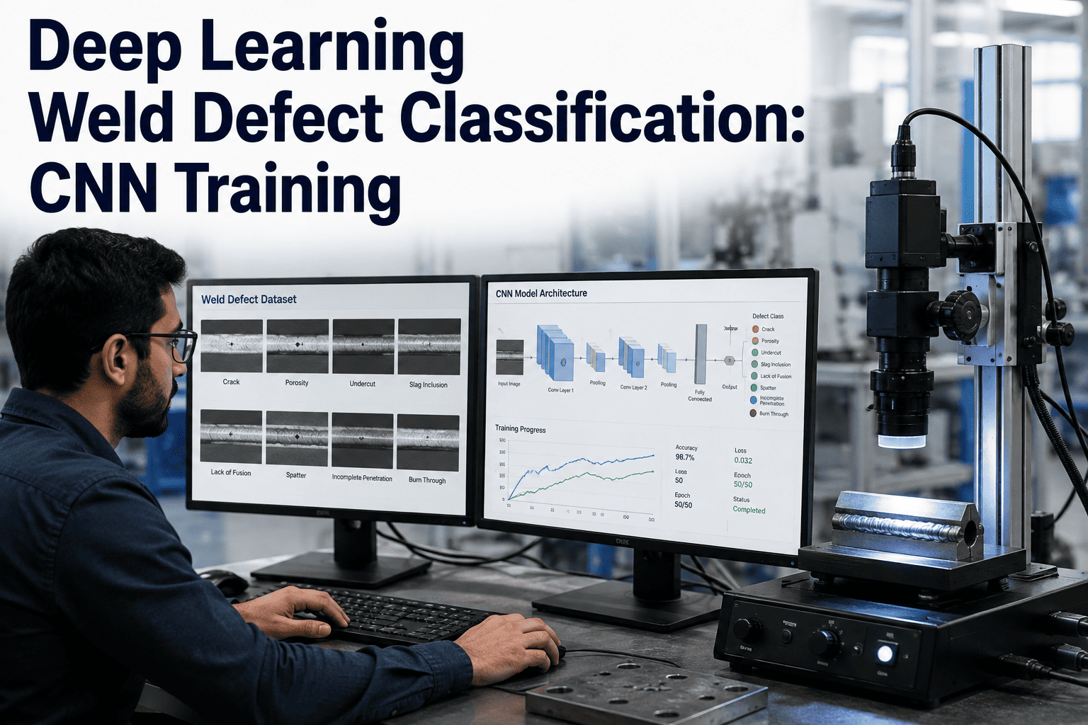
A CNN trained on a clean benchmark dataset can hit 98% accuracy in a research paper and still fail on your production line in the first week. The gap between a lab result and a working weld inspection system almost never comes down to the model architecture — it comes down to what happened before training even started: how the images were collected, how the defects were labeled, and how the team handled the fact that good welds outnumber bad ones by a wide margin. iFactory's vision inspection engine is built around that reality, training and retraining defect models on your actual production images rather than a static public dataset.
Building a CNN That Actually Classifies Weld Defects — Not Just Benchmark Images
The five-stage pipeline that separates a model that scores well on a paper from one that holds up on a real production line, plus the architecture and validation choices that determine which outcome you get.
Why Most Weld CNN Projects Stall Before They Reach Production
Ask most manufacturing teams why their in-house weld defect model underperforms and the answer is rarely "wrong architecture." It is almost always one of three upstream problems: not enough labeled defect images, defect classes so imbalanced the model learns to always predict "good weld," or a validation process that measured performance on images too similar to the training set. A CNN is a pattern-matching system — it will faithfully learn whatever pattern the data actually contains, including patterns you did not intend to teach it.
Public weld datasets are small
Some of the most cited public weld radiograph collections contain only a few dozen usable images in the welds category, forcing teams into manual cropping and re-annotation before any training can begin. Larger public sets exist, but most are narrow — built around one defect family, one imaging method, or one material.
Good welds dominate the data
On a real production line, good parts routinely outnumber defective parts by a hundred to one or more. A model trained naively on that distribution can reach a misleadingly high accuracy number by simply predicting "no defect" almost every time — while missing the rare cases that actually matter.
Lab accuracy is not production accuracy
The same ResNet50-based architecture that reached 98.75% accuracy on a clean, well-lit benchmark radiograph dataset dropped to 75.8% when tested against a private dataset made up of lower-quality, real-world images — the same model, a very different result.
Stage 1–2: Data Collection and Annotation That Holds Up in Production
Every weld CNN project starts with the same question: where do the training images come from, and how are they labeled once collected? Get this stage wrong and no amount of architecture tuning downstream will fix it. Get it right, and even a modest model architecture will perform respectably.
The practical target is a dataset that reflects the actual imaging conditions of your line — radiographic, visual, or thermographic — not a polished public collection photographed under ideal lighting. Teams that skip this step and train purely on public data consistently see the benchmark-to-production accuracy drop described above.
| Annotation Format | Structure | Best Fit | Tooling Note |
|---|---|---|---|
| YOLO TXT | Lightweight per-image text file, normalized bounding boxes | Real-time defect detection, edge deployment | Native support in modern detection architectures |
| COCO JSON | Single JSON file, supports segmentation masks | Multi-class classification with instance detail | Heavier format, strong ecosystem tooling |
| Pascal VOC XML | One XML file per image, bounding-box based | Legacy pipelines, academic benchmark compatibility | Verbose, largely superseded by YOLO TXT |
| Pixel-level masks | Per-pixel class labels | Fine-grained severity grading, crack propagation | Highest labeling cost, highest downstream precision |
Whichever format is chosen, consistency matters more than sophistication. A dataset where three different annotators labeled "lack of fusion" three different ways will teach the model an inconsistent boundary — and that inconsistency shows up as unstable predictions later, not as an obvious error anyone catches early.
Before any of that annotation work begins, it helps to separate the image sources you are actually going to draw from. Radiographic imaging remains the standard for internal defect types such as lack of penetration, porosity, and cracking, because it can reveal conditions invisible to a surface camera. Visual or HDR camera imaging is faster and cheaper to capture at scale, and works well for surface-level defects such as contamination, spatter, and misalignment. High-dynamic-range imaging in particular has been used specifically to improve the visibility of subtle surface defects that would otherwise be washed out under standard lighting. Thermographic imaging adds a third option for processes like resistance spot welding, where a defect may correlate more strongly with a heat signature during the weld than with the finished bead's appearance.
A practical annotation workflow for a manufacturing team usually looks like this: first, a domain expert — a welding engineer or quality inspector, not a data scientist — reviews a batch of images and defines the defect taxonomy in plain operational language. Second, that taxonomy gets translated into a fixed label set with clear boundary rules, ideally with reference images for each class so annotators are not making judgment calls from memory. Third, a subset of images is double-annotated by two people independently, and the disagreement rate between them is measured before scaling up. If two experienced annotators disagree on 20% of labels, the model will inherit that same 20% of noise, regardless of how sophisticated the architecture is downstream.
Stage 3: Augmentation Strategy for Imbalanced Defect Data
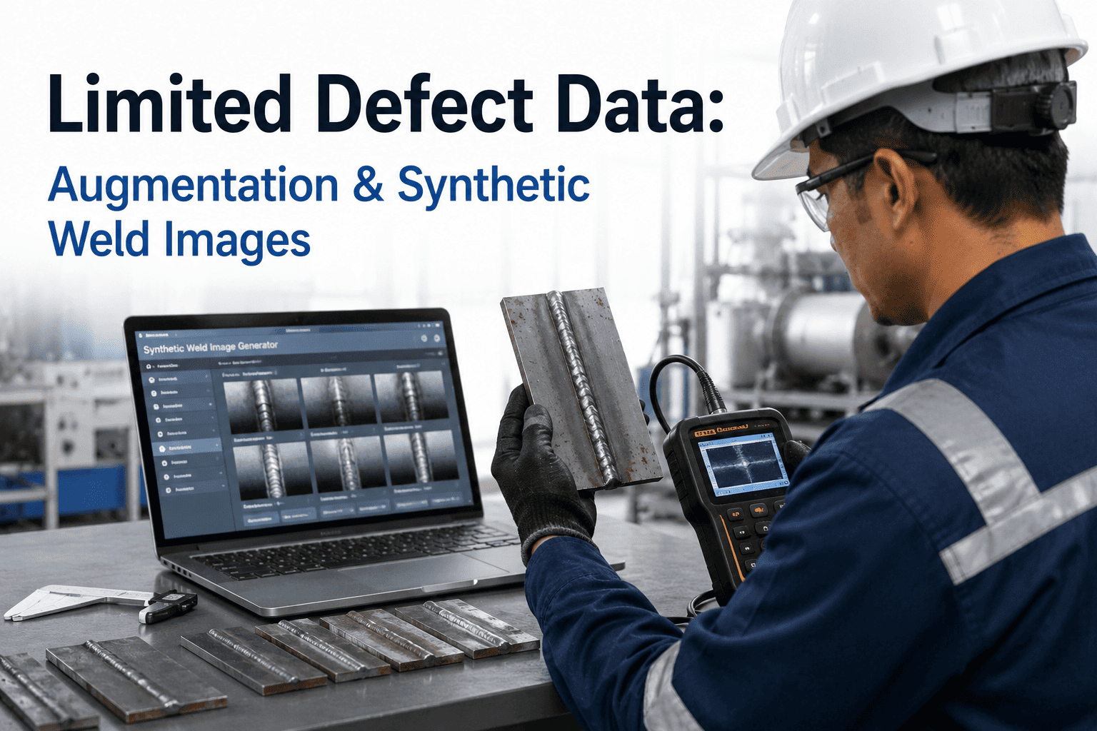
Augmentation is where most of the class-imbalance problem gets solved in practice, since collecting thousands more real defect images is rarely fast or cheap. The goal is not to make the dataset artificially large — it is to make the minority defect classes represented well enough that the model cannot shortcut its way to a high score by ignoring them.
It helps to think of augmentation as two separate jobs that are often conflated. The first job is generalization: making sure the model does not overfit to the exact lighting, angle, and background of the images it was trained on, so it still performs when a camera is repositioned or a bulb ages. The second job is balance: making sure the model sees enough examples of each defect type that it cannot achieve a high accuracy score by simply learning the base rate of "good weld" in the training set. Geometric augmentation mostly serves the first job. Oversampling and synthetic generation mostly serve the second. A training pipeline that only does one of the two will plateau — either overfitting on a narrow set of real images, or generalizing well but still ignoring rare defects because they remain statistically rare even after basic transformations.
Geometric Augmentation
Rotation, flipping, and cropping around the defect region. Cheap to apply and effective for defects like porosity or spatter that have no fixed orientation on a weld bead.
Oversampling the Minority Class
Duplicating existing minority-class defect images during training so the model sees defect examples as often as it sees "good weld" examples, rather than a hundred times less often.
GAN-Based Synthetic Generation
Generative adversarial networks trained to produce realistic synthetic defect images, used specifically to correct insufficient and unbalanced defect representation in smaller datasets.
Mosaic and MixUp
Combining multiple training images into one composite so the model learns to detect defects at multiple scales and against varied backgrounds — particularly useful for small defects like pinholes.
Your Weld Images Are Already Generating the Training Data You Need
iFactory connects to your existing inspection cameras and radiographic equipment to continuously build and refine a defect dataset from real production images — instead of starting from a static public benchmark.
Stage 4: Choosing a CNN Architecture — What the Comparisons Actually Show
Architecture selection is the stage most engineers spend the most time debating, and the stage that matters least relative to data quality. That said, the choice still affects training speed, deployment footprint, and final accuracy — so it is worth grounding in what comparative studies have actually found rather than defaulting to whichever architecture is most familiar.
| Architecture | Relative Size | Reported Behavior | Practical Fit |
|---|---|---|---|
| DenseNet121 | Moderate | Reached the highest accuracy among compared architectures in a multi-model welding defect study | Strong default when accuracy matters more than inference speed |
| ResNet50 | Large | Reached 98.75% on a clean benchmark set, but dropped sharply on lower-quality real-world images | Strong on clean data; test thoroughly on production-quality images |
| VGG16 (fine-tuned) | Large | Reached roughly 90% average accuracy across 15 unbalanced defect classes using transfer learning | Reliable transfer-learning baseline for smaller labeled datasets |
| MobileNet | Small | Included in multiple comparative studies as the lightweight option for constrained hardware | Best fit for edge deployment on line-side inspection hardware |
| Lightweight custom CNN | Smallest | Purpose-built lightweight CNNs paired with GAN-based augmentation have matched larger models while running faster | Best when inference latency on the line is the binding constraint |
Two patterns hold across nearly every comparative study in this space. First, transfer learning — starting from a network pretrained on a large general image dataset and fine-tuning it on weld images — consistently outperforms training a large architecture from scratch on a small weld dataset, since deep networks trained from scratch on limited data tend to overfit. Second, no single architecture wins outright; the right choice depends on whether the constraint is accuracy, inference speed, or deployment hardware.
The deployment context tends to settle this decision in practice more than the accuracy table does. A radiography lab reviewing images in batch after a shift has finished has very different constraints than a line-side camera system that has to classify a weld within a fraction of a second before the next part arrives. For the first case, a larger and more accurate architecture like DenseNet121 or a fine-tuned ResNet50 is usually the right call, since inference time is not the bottleneck. For the second case, a lightweight architecture such as MobileNet or a purpose-built compact CNN is often the only realistic option, because the hardware sitting at the edge of a production line rarely has the memory or compute budget of a data center GPU. Teams that pick the highest-accuracy architecture from a leaderboard without checking it against their actual hardware constraints frequently discover the mismatch only after the model is already built.
Stage 5: Validation, Cross-Checking, and Explainability
A model is only as trustworthy as its validation process. Splitting data randomly into training and test sets is not enough when defect classes are imbalanced — a random split can easily leave a rare defect type almost entirely in the training set, making the test score look better than real-world performance will be.
- Stratified cross-validation — ensures each defect class, including rare ones, is proportionally represented in every fold, rather than concentrated in one split.
- Held-out production images — a final test set built from real line images the model has never seen, not a subset of the same benchmark collection used for training.
- Computational-time analysis — measuring inference speed alongside accuracy, since a model too slow for line speed is not viable regardless of its accuracy score.
- Grad-CAM or comparable visual interpretation — generating a heatmap of which pixels drove a classification decision, so an engineer can confirm the model is actually looking at the weld defect and not an unrelated artifact in the frame.
That last point matters more than it might first appear. Explainability tooling such as Grad-CAM has been paired directly with CNN weld classifiers specifically so that a quality engineer can visually confirm the model's reasoning before trusting it on the line — turning a black-box prediction into something a human can audit.
Accuracy alone is also a misleading single number to report on an imbalanced dataset, and most rigorous studies in this space report several metrics side by side rather than one headline figure. Precision and recall broken out per defect class matter more than an overall accuracy score, because a model can post a high overall accuracy while still missing the majority of a rare but safety-critical defect type. Macro-averaged F1 score — which treats every class equally regardless of how many examples it has — is a better single-number summary than accuracy when classes are imbalanced, since it will not reward a model for simply favoring the majority class. A validation report worth trusting shows the confusion matrix directly, not just a summary accuracy percentage, so an engineer can see exactly which defect types are being confused with which.
The Benchmark-to-Production Gap, and What Closes It
The single most honest finding across recent comparative weld CNN research is this: the same model architecture, trained and evaluated the same way, can perform dramatically differently depending on image quality and source. A model can score in the high 90s on a clean benchmark set and land in the mid-70s on a private dataset of lower-quality, real-world images — a gap large enough to be the difference between a viable inspection system and one nobody trusts.
Closing that gap is less about finding a better architecture and more about continuously feeding the model real production images, retraining as new defect variants appear, and validating against the actual imaging conditions on your line rather than a static academic dataset. This is the specific gap iFactory's vision inspection pipeline is built to close — treating the model as a living system tied to your production data, not a one-time training exercise.
The mistake I see most often is a team celebrating a 98% accuracy number from a public benchmark and assuming that number will hold on their own line. It almost never does. Your welds are not the benchmark's welds — different metal, different lighting, different camera, different defect mix. The teams that succeed are the ones who treat the benchmark result as a starting hypothesis, not a finished product, and who budget real time for collecting and annotating their own defect images before they trust the model with a single reject decision.
Frequently Asked Questions
How many labeled weld defect images do I actually need to train a usable CNN?
There is no single universal number, because it depends heavily on whether you use transfer learning and how many defect classes you are trying to distinguish. Studies have shown workable classifiers built from datasets as small as a few hundred manually labeled image patches when transfer learning was used to fine-tune a network pretrained on general images, while training a large architecture from scratch typically needs far more data to avoid overfitting. A practical starting target is at least a few hundred examples per defect class, with transfer learning used to compensate for the rest. iFactory's team can help assess whether your current image volume is sufficient before you commit to a training approach.
Should I train a CNN from scratch or use transfer learning for weld defects?
For nearly all manufacturing teams, transfer learning is the better starting point. Pretrained networks such as VGG16, ResNet50, and DenseNet121 have already learned general visual features from massive image collections, and fine-tuning them on a smaller weld-specific dataset consistently outperforms training a comparable architecture from scratch on limited data. Training from scratch only becomes competitive once you have a very large, well-balanced labeled dataset of your own — which most single-plant deployments do not have at project start. Book a demo to see how iFactory handles this trade-off automatically.
How do I handle the fact that defective welds are much rarer than good welds in my data?
This class imbalance problem is one of the most common reasons in-house weld models underperform, since good parts can outnumber defective parts by a hundred to one or more on a real line. Effective countermeasures include oversampling the minority defect classes during training, generating synthetic defect examples with generative adversarial networks, and using stratified cross-validation so every fold contains a proportional share of each defect type rather than concentrating rare defects in a single split. Ignoring imbalance produces a model that scores well on paper by simply predicting "no defect" most of the time.
Why did my model's accuracy drop so much when I moved from a public dataset to my own plant's images?
This is an extremely common and well-documented pattern. Comparative research has shown the same architecture reaching accuracy in the high 90s on a clean, well-curated benchmark radiograph dataset, then dropping to the mid-70s on a private dataset made up of lower-quality, real-world images — same model class, very different result. The gap comes from differences in lighting, camera equipment, image resolution, and defect variety between the benchmark and your actual production environment. The fix is retraining and validating specifically against your own production images rather than relying on benchmark performance as a proxy.
How do I know the model is actually detecting the defect and not something else in the image?
This is exactly what explainability tools like Grad-CAM are designed to answer. Grad-CAM generates a visual heatmap over the input image showing which pixels most influenced the model's classification decision, letting a quality engineer visually confirm the model is focused on the actual defect region rather than an unrelated artifact, shadow, or background feature. Several recent weld classification studies have paired CNN architectures directly with this kind of visual interpretation specifically to build trust before deployment. iFactory surfaces this kind of visual explanation alongside every defect classification for exactly this reason.
Stop Validating Against a Benchmark. Start Validating Against Your Line.
iFactory retrains weld defect models on your actual inspection images, tracks accuracy separately for every defect class, and surfaces Grad-CAM style visual explanations your quality team can audit.