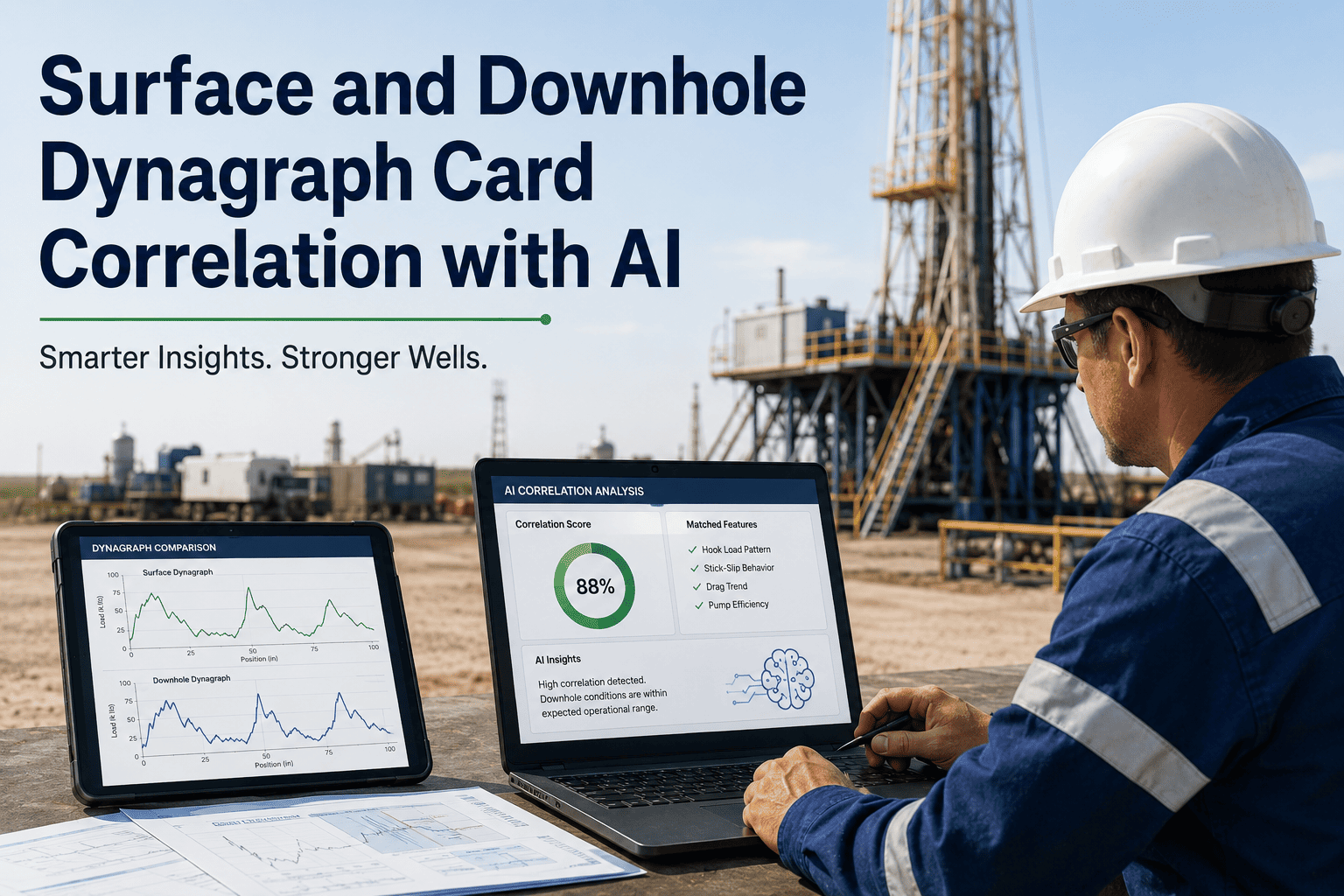
A surface dynamometer card only tells half the story. It records the load and position measured at the polished rod, at the very top of the well, while the pump itself works thousands of feet below, hidden from view and hard-wired instrumentation. For decades, engineers have leaned on the Gibbs wave equation to translate that surface signal into a predicted downhole card, and for just as long, the translation has depended on a fixed damping assumption, a manual finite-difference solve, and an analyst's trained eye reading the resulting shape. iFactory layers a machine learning correction and pattern-classification model onto that same wave equation solver, so every stroke produces a downhole card that reflects what the pump is actually doing in that well, right now, rather than what a static model assumed thirty years ago. Book a 30-minute scoping call to see your own field's surface cards converted into AI-corrected downhole diagnostics.
From Surface Stroke to Downhole Truth, Automatically
Every pumping unit already generates the data a diagnosis needs — a load cell and a position sensor riding the polished rod. The question has never been whether that data exists, but whether the translation from surface load to downhole pump behavior can be trusted. iFactory pairs a finite-difference wave equation solver with a machine learning correction layer trained on thousands of labeled surface-to-downhole card pairs, so the resulting downhole card reflects real well conditions instead of a damping factor nobody has revisited since the well was completed.
Why Surface-Only Diagnostics Fall Short
Roughly 85 to 90 percent of producing wells in the United States run on sucker-rod, or beam, lift, and nearly every one of them is monitored first through a surface card. The trouble is that a surface card only shows what happens at the top of the string. Friction, rod stretch, and wave reflection all distort the signal long before it reaches an analyst's screen, and a card that looks abnormal at surface can be perfectly normal downhole, or the reverse.
the decade S.G. Gibbs introduced the damped wave equation that still underpins most rod-pump diagnostic software today
Fourier coefficients typically needed for a classical Gibbs-method solution to converge on a stable downhole card
data points per stroke a wave equation solver needs from the surface card to reconstruct downhole load and position
of downhole misdiagnoses that trace back to a fixed damping factor that no longer matches actual well conditions
Inside the Gibbs Wave Equation
The rod string behaves like a long, slender, damped spring. Load applied at the surface does not arrive at the pump instantaneously or unchanged — it travels down the steel as a wave, stretched by inertia and dissipated by friction along the way. The damped one-dimensional wave equation is the mathematical model that describes that journey, and every downhole card computed from a surface card, whether by a 1960s Fourier solution or a modern AI-corrected pipeline, starts from this same relationship.
Six Classic Diagnostic Card Shapes
Once the downhole card is computed, the shape it traces tells a story. Trained analysts have read these shapes for generations; the pattern is a well-established taxonomy of the same handful of downhole conditions repeating across fields, formations, and pump types.
Fluid pound
A sudden, sharp load drop partway through the downstroke as the plunger free-falls through gas before striking liquid. A classic sign of overproduction relative to well inflow.
Gas interference
A rounded, gradual load transition rather than a sharp corner, caused by gas compressing in the barrel before liquid enters the pump chamber.
Worn traveling valve
Load fails to build cleanly at the start of the upstroke, since fluid leaks back through a ball or seat that no longer seals under pressure.
Worn standing valve
Load fails to hold during the downstroke, showing a card that never fully unloads because fluid is bleeding back into the tubing below.
Rod parting or unscrewing
Load collapses to near zero partway through a stroke and stays there, an unmistakable signature of a mechanical break in the string.
Tubing movement
An unanchored or loosely anchored tubing string stretches under load, distorting the card into a leaning parallelogram rather than a clean loop.
See Your Field's Cards Converted in Real Time
Bring a set of recent surface cards from your own field. iFactory runs them through the wave equation solver and the AI correction layer live on the call, and shows the resulting downhole diagnosis side by side with your analyst's read.
Manual Wave-Equation Solvers vs AI-Corrected Solvers
The wave equation itself has not changed since Gibbs and later Everitt and Jennings defined it. What has changed is how the damping term is calibrated and how the resulting card gets read — and that difference is where most of the diagnostic value now lives.
- Damping factor set once at commissioning, rarely revisited per well
- Assumes a simple, vertical, single-taper rod string unless manually reconfigured
- Downhole card shape read and classified by an individual analyst
- Diagnosis quality depends on that analyst's experience and current caseload
- Recalculated only when someone actively pulls and reviews the card
- Damping factor recalibrated continuously against fluid level and stroke data
- Deviated and tapered rod strings modeled automatically from configuration data
- Card shape matched against a trained pattern library in seconds
- Consistent diagnosis regardless of analyst caseload, shift, or fatigue
- Every stroke reprocessed automatically as new surface data streams in
The iFactory AI Dynagraph Pipeline
Five stages carry a raw surface stroke to a routed diagnostic alert, all inside the same cycle time as the pump's own stroke rate.
Surface data capture
Load cell and position sensor readings from the polished rod stream to the edge gateway every stroke, time-stamped and tied to well and pumping unit configuration.
Wave equation solve
A finite-difference Everitt-Jennings solver computes the baseline downhole card from surface position and load, using rod-string geometry and material properties per well.
ML damping correction
A trained model adjusts the damping factor stroke by stroke against fluid level, production trend, and historical card shape, instead of holding it fixed.
Pattern classification
The corrected downhole card is matched against a labeled library covering fluid pound, gas interference, valve wear, rod failure, and tubing movement, among others.
Diagnostic alert & trend
The classified result is pushed to the production dashboard and trended over time, with alerts routed to the responsible engineer before the condition worsens.
Downhole Card Calculation Methods Compared
The wave equation has been solved several different ways since Gibbs first published his method, each suited to different rod-string complexity and diagnostic scale.
What Changes After Deployment
Figures from typical rod-lift fleets within the first 120 days of running AI-corrected downhole diagnostics across their well count.
The 8-Week AI Dynagraph Rollout
One field, your existing surface card history, and a fixed timeline from kickoff to a validated diagnostic dashboard.
Collect rod-string configuration, pump specifications, and historical surface cards per well.
Configure the Everitt-Jennings solver per well and establish a baseline damping factor for each.
Train the pattern classifier on your labeled historical cards and known failure events.
Run in parallel against analyst diagnoses, tune thresholds, and sign off for full deployment.
Our team used to pull surface cards once a week per well and spend two full days working through the backlog before anyone saw a diagnosis. By the time we flagged a fluid pound condition, the well had usually been pounding for days. Now the corrected downhole card updates every stroke, the pattern is flagged the moment it starts trending, and our production engineers spend their time acting on diagnoses instead of producing them.
wells a single analyst can now review weekly with AI-corrected diagnostics
typical turnaround from stroke capture to a routed diagnostic alert
reduction in unplanned workovers within the first four months of deployment
Frequently Asked Questions
Does the AI replace the wave equation solver, or work alongside it?
It works alongside it. The finite-difference Everitt-Jennings solver still does the core physics work of turning surface position and load into a predicted downhole card, exactly as it has for decades. What the machine learning layer adds is continuous recalibration of the damping factor and automatic classification of the resulting card shape, rather than a fixed assumption reviewed once a year. Talk to a specialist about how the two layers are split on your existing well configuration.
Which rod string configurations can the solver handle, only simple vertical wells?
No. Tapered rod strings, deviated wellbores, and non-anchored tubing are all supported, since the finite-difference method discretizes the string into segments with their own length, area, and material properties rather than assuming a single uniform rod. Deviated and complex geometries typically need more segments and a longer initial calibration, which the onboarding process accounts for per well.
How accurate is the AI-corrected downhole card compared to a physical bottom-hole gauge?
Wave-equation-derived cards have long been the accepted substitute for physical downhole measurement, since running a gauge on every well is not economically practical at fleet scale. The AI correction layer improves on a static-damping solve by continuously tuning the damping term against fluid level and production data, narrowing the gap between the predicted card and what a gauge would actually record on wells where both are available for comparison.
Can it automatically detect conditions like fluid pound and gas interference?
Yes. The pattern classification stage compares every corrected downhole card against a labeled library that covers fluid pound, gas interference, worn traveling and standing valves, rod parting, and tubing movement, among other conditions. Each classification comes with a confidence level, and borderline or trending cases are flagged for an engineer to review rather than silently passed through.
How long does it take to get AI dynagraph diagnostics running across our field?
A single-field pilot typically runs eight weeks from kickoff, covering well inventory, solver calibration, model training on your own historical cards, and a validated dashboard rollout. Fleet-wide expansion after a successful pilot moves faster, since the solver configuration and classification model are already built. Book a scoping call to get a timeline specific to your well count.
See AI-Corrected Downhole Cards on Your Own Wells
Book a 30-minute scoping call and bring a set of recent surface cards from your field. iFactory runs the wave equation solve and the AI correction live, shows the resulting diagnosis, and builds a fixed-timeline pilot proposal for your well count.