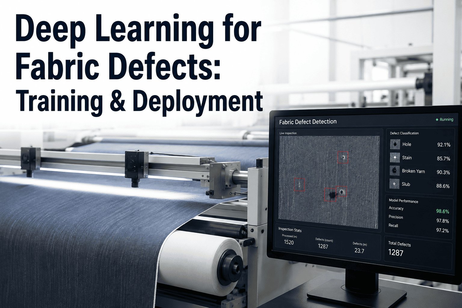
A convolutional neural network that achieves 98% validation accuracy in a Jupyter notebook and a convolutional neural network that reliably classifies fabric defects on a production line running at 40 meters per minute are, in practice, two different engineering problems that happen to share the same underlying architecture. The gap between them is filled with decisions that rarely appear in academic papers on textile defect classification: which backbone architecture actually fits the latency budget imposed by line speed and camera field of view, how to build a training dataset that captures the true distribution of defect types without spending months manually annotating fabric, and how to compress and deploy a model onto edge hardware that has to run continuously in a production environment rather than a GPU server. This is a practical engineering reference for building and deploying deep learning fabric defect classification systems that actually work in production — not just in a benchmark. Book a technical session with the iFactory computer vision team to discuss architecture and deployment specifics for your fabric type and line configuration.
Manual Inspection · Deep Learning for Fabric Defect Classification
Training and Deploying Deep Learning Models for Fabric Defect Classification: An Engineering Reference
CNN architecture selection, data augmentation strategy specific to fabric defects, training methodology, and edge deployment under real production line speed constraints — the full pipeline from problem framing to production validation.
01
Input
Line-scan or area camera frames · RGB or multispectral
→
02
Backbone
CNN feature extractor · ResNet / EfficientNet / MobileNet
→
03
Feature Maps
Multi-scale spatial features · FPN for size variance
→
04
Detection Head
Classification + localization · Anchor-based or anchor-free
→
05
Edge Inference
Quantized · TensorRT/ONNX · <30ms per frame
Problem Framing
Classification vs. Detection vs. Segmentation — Choosing the Right Task Formulation
Before selecting an architecture, the fabric defect problem must be correctly framed as one of three distinct computer vision task types, because the choice determines the entire downstream pipeline — labeling methodology, architecture family, loss function, and evaluation metrics all follow from this decision.
| Task Type |
Output |
Labeling Effort |
When to Use |
Typical Architecture |
| Image classification |
Single label per fabric patch/tile |
Low — patch-level pass/fail or defect-type tag |
Simple pass/fail gating on tiled inspection zones |
ResNet, EfficientNet as standalone classifier |
| Object detection |
Bounding box + class per defect |
Medium — box annotation per instance |
Locating and counting discrete defects (broken ends, snarls) |
YOLO, Faster R-CNN, RetinaNet |
| Semantic/instance segmentation |
Pixel-level mask per defect |
High — pixel-precise mask annotation |
Extent-sensitive defects (weft bars, width variation, stains) |
U-Net, Mask R-CNN, DeepLabv3+ |
Most production fabric inspection systems use object detection as the primary task — it provides the location and classification information needed for downstream severity scoring while requiring substantially less annotation effort than pixel-level segmentation, which is typically reserved for defect types where extent (not just presence) directly determines severity, such as weft bars or shade variation.
Architecture Selection
Backbone Comparison — Accuracy, Latency, and the Trade-off That Actually Matters
Architecture selection for fabric defect detection is dominated by a single constraint that academic benchmarks rarely emphasize: inference latency must fit within the time budget imposed by line speed and camera field of view. A line running at 40 meters per minute with a 500mm camera field of view produces a new frame roughly every 750 milliseconds — but the practical inference budget is far tighter than this suggests once buffering, multi-camera coverage, and safety margin are accounted for, typically requiring per-frame inference under 30 to 50 milliseconds on the target edge hardware.
ResNet-50 / ResNet-101
mAP: High
Latency: Medium-High
Params: 25–44M
The reference standard for accuracy benchmarking. Excellent feature extraction quality for subtle texture-based defects (weft streaks, low-relief snarls) but heavier than ideal for real-time edge deployment without aggressive quantization. Best suited as the backbone when a dedicated GPU or high-performance edge accelerator is available at the inspection point.
EfficientNet-B0 to B3
mAP: High
Latency: Medium
Params: 5–12M
Compound scaling (depth, width, resolution scaled together) produces a strong accuracy-to-parameter ratio, making the smaller variants (B0, B1) a common production choice when balancing detection quality against edge inference budget. B0 in particular is a frequent default starting point for new fabric defect projects given its favorable trade-off curve.
MobileNetV3 / MobileNetV2
mAP: Medium
Latency: Low
Params: 2–6M
Depthwise separable convolutions dramatically reduce parameter count and inference cost, purpose-built for mobile and edge deployment. Accuracy on subtle, low-contrast defect types (weft streaks, minor pattern deviation) is measurably lower than ResNet or EfficientNet backbones — the right choice when latency headroom is the binding constraint and defect types are predominantly high-contrast (broken ends, holes, obvious pattern breaks).
YOLOv8 / YOLOv9 (full pipeline)
mAP: High
Latency: Low
Params: Varies by scale
Single-stage detector architecture (backbone + neck + head unified) rather than a separate backbone-plus-detector assembly, optimized end-to-end for real-time detection speed. The current default choice for production fabric inspection systems where both accuracy and inference speed matter, offering multiple scale variants (nano through extra-large) to match available edge compute budget directly.
Data and Augmentation Strategy
Building a Training Dataset That Reflects Real Defect Distribution — Not Just What's Easy to Collect
The single most common cause of production underperformance in fabric defect models is not architecture choice — it is a training dataset that does not reflect the true production distribution of defect types, severities, and fabric conditions. Rare but commercially significant defect types are systematically underrepresented in naturally collected data because, by definition, they occur infrequently. Data strategy must deliberately correct for this rather than simply collecting whatever appears during normal production monitoring.
Class Imbalance Correction
Common defects (broken ends, obvious weft bars) will naturally dominate a randomly collected dataset while rare-but-critical defects (specific pattern misalignment types, subtle contamination) remain underrepresented. Address through targeted collection campaigns for underrepresented classes, class-weighted loss functions during training, and oversampling of minority-class examples in each training batch — never simply training on the naturally occurring class distribution without correction.
Fabric-Specific Augmentation
Standard image augmentation (rotation, flip, color jitter) applies reasonably well to fabric imagery, but fabric-specific augmentations improve generalization further: simulated lighting variation matching actual production line illumination conditions, synthetic texture noise matching the fiber-level texture variation across fabric types, and controlled synthetic defect injection (compositing known defect signatures onto clean fabric backgrounds) to expand rare-class coverage without requiring physical defective samples.
Multi-Fabric-Type Generalization
A model trained exclusively on one fabric weave and color will generalize poorly to a different weave structure or dark-colored fabric, even for the same defect type, because the defect's visual signature against the background changes substantially. Production deployments spanning multiple fabric types require either a sufficiently diverse training set spanning the target fabric range, or a fabric-type-conditioned model architecture, or separate models per major fabric category — the correct choice depends on how much visual diversity the model actually needs to handle.
Annotation Quality Control
Inter-annotator agreement on defect boundary and classification directly limits model performance — a model cannot exceed the consistency of the labels it was trained on. Establishing the defect catalog with clear visual criteria before annotation begins, running periodic inter-annotator agreement checks during the labeling process, and routing ambiguous cases to a senior reviewer rather than leaving classification to annotator judgment alone are all necessary quality controls, not optional refinements.
Discuss Your Specific Architecture and Deployment Constraints
iFactory's Computer Vision Team Reviews Your Line Speed, Camera Configuration, and Defect Catalog to Recommend the Right Model Architecture
Architecture selection and deployment configuration are highly specific to your line speed, camera setup, and defect distribution — there is no universal correct answer. iFactory's technical assessment reviews your actual production constraints and provides a specific architecture and deployment recommendation, not a generic best-practices document.
Training Methodology
Transfer Learning, Loss Function Design, and Validation Strategy for Fabric Defects
Training methodology for fabric defect models benefits significantly from transfer learning given the typically limited size of fabric-specific labeled datasets relative to what training a network from random initialization would require. The training approach below reflects current practice for production-oriented fabric defect models.
01
Pretrained Backbone Initialization
Initialize the backbone with ImageNet-pretrained weights rather than random initialization — even though fabric imagery differs substantially from ImageNet's natural image distribution, the low-level features learned (edges, textures, gradients) transfer usefully and substantially reduce the labeled data volume required to reach production-quality accuracy. Full fine-tuning of the entire backbone typically outperforms freezing early layers, given sufficient labeled fabric data (generally 2,000+ annotated defect instances per class).
02
Loss Function Design for Severity-Weighted Detection
Standard object detection loss functions (classification loss plus bounding box regression loss) treat all classes equally, but fabric defect severity classes are not equally important to get right — a critical defect misclassified as cosmetic carries far higher business cost than the reverse error. Incorporating class-weighted loss terms that penalize under-detection of high-severity classes more heavily than over-detection produces a model whose error pattern better matches actual business risk tolerance.
03
Multi-Scale Training for Defect Size Variance
Fabric defects range from sub-millimeter texture anomalies to full-width bars spanning the entire fabric — a single-scale training approach will systematically underperform on whichever end of this size range receives less representation. Feature Pyramid Network (FPN) architectures, combined with multi-scale training (randomly varying input resolution during training), improve detection consistency across this wide size range.
04
Validation Strategy — Production-Representative Splits
Random train/validation splitting risks data leakage when multiple frames from the same fabric roll or the same defect instance (captured across consecutive frames) end up in both training and validation sets, producing an artificially inflated validation accuracy that does not reflect true generalization. Split by production lot, roll, or time period rather than randomly by individual frame, ensuring the validation set genuinely tests generalization to unseen fabric rather than memorization of near-duplicate frames.
Edge Deployment
From Trained Model to Production Inference — Quantization, Hardware Selection, and Latency Budgets
A model that performs well in validation must be converted, optimized, and deployed onto edge hardware capable of sustaining the required inference rate continuously in a production environment — a distinct engineering phase with its own failure modes separate from model training itself.
| Deployment Step |
Purpose |
Typical Tooling |
Common Pitfall |
| Model quantization |
Reduce precision (FP32 → INT8/FP16) for faster inference and lower memory footprint |
TensorRT, ONNX Runtime, TFLite |
Naive quantization without calibration data degrades accuracy on subtle defect classes disproportionately |
| Graph optimization |
Fuse operations, eliminate redundant computation in the inference graph |
ONNX graph optimizer, TensorRT builder |
Custom layers or operations not supported by the target runtime require manual reimplementation |
| Hardware selection |
Match compute capability to required inference throughput |
Industrial edge GPU (Jetson class), dedicated inference accelerator |
Selecting hardware based on peak theoretical throughput rather than sustained thermal-limited throughput in a production enclosure |
| Pipeline integration |
Camera capture → preprocessing → inference → post-processing → decision output |
GStreamer, DeepStream, custom capture pipeline |
Preprocessing (resize, normalize) treated as free — often consumes meaningful latency budget if not optimized |
A realistic edge inference budget for a fabric inspection line running 30–50 meters per minute with a single camera covering the full width typically allocates 15–25ms for image preprocessing, 20–35ms for model inference, and 5–10ms for post-processing and decision logic — placing the total pipeline latency target at 40 to 70 milliseconds per frame, with margin against the theoretical maximum frame interval to accommodate processing jitter.
Production Validation
Confirming the Model Actually Works Before Full Deployment — Shadow Mode and Confidence Calibration
The final phase before full production deployment validates that the model's real-world performance matches its validation-set performance under actual production conditions, and establishes the confidence thresholds that determine automated versus human-reviewed classification decisions.
Shadow Mode Deployment
The model runs alongside existing inspection (manual or a prior system) without its outputs driving any production decision, logging predictions for comparison against the ground truth established by the existing process. This phase, typically running 2 to 6 weeks depending on production volume, surfaces any gap between validation-set accuracy and real production performance before the model has any operational authority.
Confidence Threshold Calibration
Raw model confidence scores are not inherently well-calibrated probabilities — a model reporting 90% confidence is not necessarily correct 90% of the time. Post-hoc calibration techniques (temperature scaling, Platt scaling) adjust raw confidence outputs to better reflect true prediction reliability, which directly determines where the high-confidence auto-classification, medium-confidence review, and low-confidence escalation thresholds should be set for the specific deployed model.
Drift Monitoring Post-Deployment
Production conditions change after deployment — new fabric lots, seasonal lighting variation, camera lens degradation — and model performance can degrade gradually without any explicit failure event. Ongoing monitoring of prediction confidence distribution, human-override rate on flagged cases, and periodic re-validation against freshly sampled ground truth data detects this drift before it becomes a significant quality risk.
Model Performance KPIs
Six Metrics That Define Production-Ready Fabric Defect Model Performance
Mean Average Precision (mAP)
Target: >0.85 @ IoU 0.5
Standard object detection accuracy metric averaged across defect classes. Should be evaluated per-class as well as in aggregate, since aggregate mAP can mask poor performance on rare but critical defect categories that are underrepresented in the evaluation set.
Per-Frame Inference Latency
Target: within line-speed budget
End-to-end latency from frame capture to classification output, measured on the actual deployed edge hardware under production thermal and load conditions — not on a development GPU. The hard constraint that determines deployment feasibility regardless of model accuracy.
False Negative Rate — Critical Class
Target: <2%
Rate of missed detections specifically for critical-severity defect classes — the metric with the highest business consequence, since a missed critical defect can reach the customer undetected. Tracked separately from overall false negative rate, which averages across severity classes and can obscure critical-class performance.
Calibration Error (ECE)
Target: <5%
Expected Calibration Error — measures how well raw model confidence scores match actual empirical accuracy. Directly determines the reliability of the confidence-based routing (auto-classify / human review / escalate) that governs production workflow decisions.
Human Override Rate
Trend: decreasing, stabilizing <10%
Percentage of medium and low-confidence model predictions that human review overturns. A high or rising rate indicates either a training data gap for the classes being overridden or a genuine shift in production conditions the model has not adapted to.
Model Drift Score
Monitor continuously
Statistical distance between the confidence and class distribution of recent production predictions versus the training/validation distribution baseline. Rising drift score is a leading indicator that retraining or recalibration is needed before accuracy visibly degrades in production metrics.
From the Engineering Team
“
The pattern I have seen repeat across nearly every fabric defect model deployment I have been involved in is that teams spend the majority of their time on architecture selection and hyperparameter tuning, and far too little time on the data pipeline and deployment engineering that actually determine whether the system works in production. A ResNet-50 and an EfficientNet-B1 trained on a well-constructed, properly balanced dataset with representative augmentation will both perform respectably — the choice between them matters far less than most teams initially assume. What matters enormously is whether the training data actually reflects the true production distribution of defect types and severities, whether the validation split genuinely tests generalization rather than memorization, and whether the deployed inference pipeline sustains its required latency under real production thermal and load conditions rather than the idealized conditions of a development GPU. I tell every team starting a fabric defect model project the same thing: budget more time for data engineering and deployment validation than you initially think you need, and treat architecture selection as a solved problem you can revisit later if performance genuinely demands it. Almost nobody follows this advice on the first project. Almost everyone wishes they had by the end of it.
Kwame Osafo-Lindström
Computer Vision Engineer · Industrial Inspection Systems Specialist · 14 years building deployed deep learning systems for manufacturing quality inspection · Former Senior ML Engineer, industrial vision systems provider · Contributor to open-source object detection tooling for manufacturing applications
Engineering Team Questions
Deep Learning for Fabric Defect Classification — Frequently Asked
How much labeled training data do we actually need to build a production-ready fabric defect detection model?
Using transfer learning from an ImageNet-pretrained backbone, a reasonable production-quality starting point requires approximately 500 to 1,000 annotated instances per defect class for common defect types, and this can be somewhat lower (200 to 400 instances) for high-contrast, visually distinctive defects like broken ends or holes, while requiring more (1,500+ instances) for subtle, low-contrast defects like weft streaks or minor pattern deviation where the visual signal-to-noise ratio is inherently lower. These figures assume reasonably consistent, well-annotated data — inconsistent annotation quality effectively raises the required volume since the model must learn to average over labeling noise. Synthetic data augmentation, including controlled defect injection compositing, can meaningfully reduce the volume of physically collected and manually annotated rare-class examples needed, though it should supplement rather than fully replace real production data given the risk of synthetic-to-real domain gap. For a data volume assessment specific to your defect catalog and current data availability,
book a technical session with the iFactory computer vision team.
Should we use a single unified model across all our fabric types, or separate models per fabric category?
This decision depends primarily on how visually similar the fabric types are and how much labeled data is available per category. A single unified model trained across diverse fabric types (different weaves, colors, textures) generally requires substantially more training data to achieve equivalent per-category accuracy compared to specialized models, because the network must learn a feature representation general enough to handle the full visual diversity rather than specializing to one fabric's specific characteristics. In practice, a hybrid approach often works well: a shared backbone (potentially frozen or lightly fine-tuned) that has learned general fabric-relevant low-level features, with fabric-category-specific detection heads or light fine-tuning applied for each major fabric family. This captures much of the efficiency benefit of a unified model — a single feature extraction backbone to maintain — while preserving per-category specialization where it matters most for accuracy. The decision threshold in practice: if you have fewer than roughly 3 to 5 fabric categories with meaningfully different visual characteristics and adequate data per category, separate models are usually simpler to build and maintain reliably; beyond that, the hybrid shared-backbone approach typically becomes worthwhile.
What edge hardware is actually necessary to run fabric defect inference at typical production line speeds?
Hardware requirements scale with the specific model architecture, input resolution, and number of camera streams requiring simultaneous inference, but a practical mid-range configuration for a single high-resolution camera stream running a compact architecture (MobileNetV3-based or YOLOv8-nano/small scale) at typical textile line speeds is achievable on an NVIDIA Jetson Orin class edge device or equivalent, without requiring a full discrete GPU server. Higher-accuracy architectures (ResNet-50 backbone, YOLOv8-large scale) or multi-camera configurations covering full fabric width with multiple simultaneous streams push hardware requirements toward a dedicated edge server with a discrete GPU or multiple inference accelerator cards. The correct sizing exercise measures actual sustained inference latency on candidate hardware using the specific trained model — theoretical hardware specifications and vendor-published benchmark numbers are directional guides only, not a substitute for measuring your specific model on your specific hardware under realistic thermal and load conditions.
Contact our support team for a hardware sizing recommendation specific to your architecture and throughput requirements.
How do we handle the class imbalance problem when some defect types occur extremely rarely in normal production?
Severe class imbalance — where critical but rare defect types may occur in fewer than 1 in 10,000 fabric samples during normal production — requires a multi-pronged strategy rather than a single technique. First, deliberately curate a collection campaign specifically targeting the rare classes, potentially using historical archived samples, deliberately induced defects on scrap material for training purposes, or samples sourced from other facilities producing similar fabric where the rare defect occurs more frequently. Second, apply class-weighted loss functions during training that penalize errors on rare classes more heavily, preventing the model from effectively ignoring rare classes to optimize aggregate accuracy dominated by common classes. Third, use targeted data augmentation and synthetic defect compositing specifically to expand the effective rare-class training set beyond what was physically collected. Fourth, consider a cascade or ensemble approach where a separate, specifically-tuned detector for the rare critical class runs alongside the primary multi-class detector, since a specialized binary detector for a single rare-but-critical class can sometimes achieve better sensitivity than expecting a single multi-class model to handle both common and extremely rare classes well simultaneously.
How often does a production fabric defect model need to be retrained, and what triggers a retraining cycle?
Retraining cadence should be triggered by evidence of performance drift rather than a fixed calendar schedule, though most production deployments benefit from a baseline scheduled review (typically quarterly) supplemented by event-triggered retraining. Scheduled reviews assess accumulated human-review-confirmed classifications since the last training cycle, checking whether the model's error pattern has shifted in ways suggesting a retraining benefit. Event-triggered retraining is warranted by: a significant new fabric type or product line entering production that the current training data does not adequately represent, a measurable rise in the drift monitoring metrics described in the production validation section, a change in camera hardware, lighting, or physical inspection point configuration that alters the visual characteristics of captured frames, or accumulation of a substantial volume of new human-confirmed labels (particularly for previously underrepresented classes) that would meaningfully improve the training set. The retraining process itself should reuse the established data pipeline and validation methodology rather than starting from scratch, incorporating the newly accumulated production data alongside the original training set.
Book a session to discuss a retraining governance framework for your specific deployment.
From Notebook Accuracy to Production Reliability
Get a Model Architecture and Deployment Plan Built for Your Actual Line Speed and Fabric Types
iFactory's computer vision engineering team builds and deploys production fabric defect detection systems — from architecture selection matched to your specific latency budget, through data pipeline and augmentation strategy, to edge deployment and confidence calibration validated in shadow mode before going live. Every recommendation is grounded in your actual line speed, camera configuration, and defect catalog, not generic best practices.